
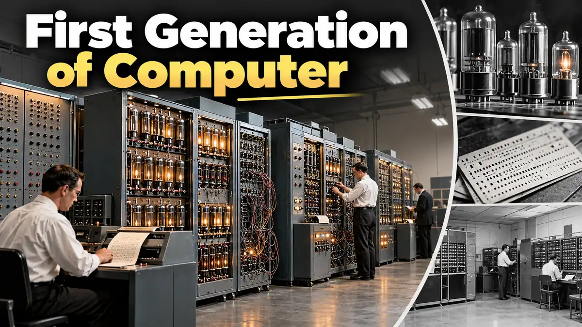

The first generation of computer marked the beginning of practical electronic digital computing. These machines were enormous, expensive, power-hungry, and difficult to program, yet they transformed calculations that previously demanded extensive human effort.
Most first-generation computers relied on vacuum tubes for electronic switching and used technologies such as punched cards, paper tape, magnetic drums, magnetic tape, mercury delay lines, and machine-language instructions. The era is commonly associated with the 1940s through the mid-1950s, although exact generation dates vary between historical classifications.
Quick answer: The first generation of computer refers to early electronic computers built mainly during the 1940s and 1950s using vacuum tubes for logic and circuitry. Famous examples include ENIAC, EDSAC, EDVAC, UNIVAC I, IBM 701, and IBM 650. They were large, costly, power-intensive machines programmed at a very low level.
What Is the first generation of computer?
The first generation of computer describes the earliest era in which electronic components—particularly vacuum tubes—became central to digital computing.
Before electronic computers, many calculating systems depended heavily on mechanical components or electromechanical relays. Vacuum tubes made much faster electronic switching possible and helped establish electronic digital computation as a practical technology.
A vacuum tube could control electrical signals and serve as part of circuits representing and processing information. Thousands of these components could be connected to construct arithmetic, control, and memory-related circuitry.
The machines were revolutionary for their time, but they were nothing like today’s laptops and smartphones. Some occupied large rooms, required substantial electrical power and cooling, and needed specialized teams to operate and maintain them.
The first-generation label should also be understood as a historical classification, not a perfectly defined period. Some educational sources use roughly 1940–1956, while historical accounts describe the first generation more generally as the vacuum-tube era beginning in the mid-1940s.
Why were they called first-generation computers?
Computer generations classify major stages of computing according to dominant technologies.
A simplified progression is:
| Generation | Key Hardware Technology | General Development |
|---|---|---|
| First generation | Vacuum tubes | Electronic digital computing |
| Second generation | Transistors | Smaller, cooler, more reliable systems |
| Third generation | Integrated circuits | Multiple electronic components integrated onto chips |
| Fourth generation | Microprocessors | CPUs placed on highly integrated chips |
| Later-generation concepts | Advanced integration and AI-oriented computing | Increasing automation and intelligent computing |
The defining hardware technology of the first generation was therefore the vacuum tube, while the transition toward transistor-based machines is normally associated with the second generation.
History of the first generation of computer
The first generation did not begin with one machine appearing overnight. It emerged from several wartime and postwar computing projects in the United States and Europe.
Military calculations, scientific research, cryptography, engineering, and large-scale data processing created strong demand for machines capable of performing calculations more rapidly and automatically.
Machines including Colossus, ENIAC, the Manchester Baby, EDSAC, EDVAC, UNIVAC I, IBM 701, and IBM 650 represent different milestones within this broader period.
ENIAC and electronic general-purpose computing
One of the best-known early machines was ENIAC, the Electronic Numerical Integrator and Computer.
Engineers J. Presper Eckert and John Mauchly developed ENIAC at the University of Pennsylvania during the 1940s. Smithsonian records date its development to 1943–1946.
ENIAC contained roughly 18,000 vacuum tubes and weighed about 30 tons according to commonly cited historical accounts.
Those specifications show why first-generation computers were so physically demanding. Thousands of electronic components had to be powered, cooled, connected, tested, and repaired.
Programming ENIAC initially differed greatly from writing software today. Setting up a new problem involved configuring switches and cable connections rather than simply loading a modern program from storage.
The stored-program breakthrough
A major problem with early electronic computing was not simply calculation speed. It was programming.
If changing a task required extensive physical reconfiguration, the computer could calculate quickly once configured but still be cumbersome to use.
The stored-program idea changed that.
Instead of treating a program mainly as a physical configuration, instructions could be represented electronically and stored in memory. The EDVAC project and John von Neumann’s widely circulated First Draft of a Report on the EDVAC became important parts of the development and spread of stored-program architecture.
This distinction is crucial because not every first-generation computer worked in exactly the same way.
Manchester Baby
The Manchester Small-Scale Experimental Machine, commonly called the Manchester Baby, successfully demonstrated stored-program computing before EDSAC. It was primarily an experimental system rather than a computer intended to provide a regular computing service.
That difference explains why several different machines are described as “first” computers in different contexts.
A machine can be first according to one criterion—such as demonstrating stored-program operation—without being first according to another, such as becoming a practical general-purpose computing service.
EDSAC
The Electronic Delay Storage Automatic Calculator (EDSAC) was developed at the University of Cambridge under Maurice Wilkes.
EDSAC successfully ran programs on May 6, 1949. Cambridge describes it as the first practical general-purpose electronic stored-program computer of its kind, capable of holding both instructions and data in memory.
EDSAC used vacuum tubes for logic, punched paper tape for input, a teleprinter for output, and mercury delay lines for memory.
This highlights an important historical detail often lost in simplified descriptions: not every first-generation computer used magnetic drums as its main memory.
EDVAC
EDVAC, or Electronic Discrete Variable Automatic Computer, was designed as a stored-program computer and represented another major step beyond ENIAC.
Its design was binary rather than ENIAC’s decimal approach, and the EDVAC project became closely connected with the development of stored-program architecture.
The concept of storing instructions in electronic memory greatly influenced subsequent computer architecture.
UNIVAC I and commercial computing
The UNIVAC I, or Universal Automatic Computer I, helped move electronic computing beyond experimental, scientific, and military projects toward large-scale administrative and commercial data processing.
Eckert and Mauchly’s company developed the system before becoming part of Remington Rand. The first UNIVAC I was delivered to the U.S. Census Bureau in 1951.
UNIVAC demonstrated that electronic computers could process large volumes of organizational data, not merely solve specialized mathematical problems.
IBM 701
Another significant first-generation machine was the IBM 701, originally known as IBM’s Defense Calculator.
IBM began its development in 1951 and announced the machine in April 1952. It was designed as a general-purpose electronic system capable of handling demanding scientific and engineering calculations.
The 701 helped establish IBM as a major participant in the emerging electronic computer industry.
IBM 650
The IBM 650 became one of the commercially important vacuum-tube computers of its era.
Unlike some machines that used other forms of electronic memory, the IBM 650 relied heavily on magnetic drum memory. Historical descriptions of drum storage note that early IBM 650 configurations held up to 2,000 ten-digit words, with later configurations expanding capacity.
Together, systems such as UNIVAC I, IBM 701, and IBM 650 showed that electronic computing was becoming an industry rather than remaining solely an experimental research field.
Characteristics of first generation computers
Although individual machines differed considerably, several characteristics are strongly associated with first-generation computing.
1. Vacuum tubes were the core electronic technology
The most recognizable feature was the use of vacuum tubes, also known as thermionic valves.
These components performed electronic switching and amplification functions that later generations accomplished with transistors and integrated circuits.
Vacuum tubes worked, but they occupied far more space and consumed considerably more energy than later semiconductor components.
2. Computers were physically large
Thousands of components, wiring connections, power systems, input/output equipment, and memory hardware made many early computers extremely large.
“Computer” therefore referred not to a small box sitting on a desk but often to an installation distributed across cabinets or an entire room.
EDSAC, for example, weighed about two tons and occupied a room at Cambridge University’s Mathematical Laboratory.
3. Electricity consumption was high
Vacuum-tube circuitry required substantial electrical power.
More power also meant more heat. Cooling and ventilation therefore became important engineering requirements for large electronic computer installations.
This increased both operating costs and infrastructure requirements.
4. Heat generation was a major challenge
Heat was one of the practical weaknesses of vacuum-tube systems.
Thousands of powered electronic components generated considerable heat, while component failures could interrupt operation and require maintenance.
This relationship between power, heat, reliability, and maintenance is one reason transistor technology later represented such an important improvement.
5. Programming was difficult
Early computer programming was much closer to the machine’s hardware than modern software development.
Machine instructions were represented at a very low level, and some early systems required physical configuration using switches, plugboards, or wiring.
Later stored-program computers dramatically improved this process by keeping instructions in memory.
6. Machine language was fundamental
First-generation programming was strongly associated with machine language, the low-level instructions directly understood by a computer’s hardware.
There were no modern graphical interfaces, web browsers, application stores, or development environments.
Programmers needed detailed knowledge of the particular machine they were operating.
7. Punched cards and paper tape were widely used
Input/output methods differed between systems, but punched cards and punched paper tape were common technologies.
Information could be encoded by patterns of holes and then mechanically or electronically read by equipment connected to the computer.
Output might be produced through printers or teleprinters rather than modern screens.
EDSAC, for example, used five-hole punched paper tape for input and a teleprinter for output.
8. Memory capacity was extremely limited by modern standards
First-generation computers had tiny storage capacities compared with today’s devices.
However, saying that all first-generation machines simply “used magnetic drums” is inaccurate.
Different machines used different technologies, including:
- Magnetic drums
- Magnetic tape
- Mercury acoustic delay lines
- Williams electrostatic storage tubes
- Other experimental electronic storage methods
Magnetic drums became important in machines such as the IBM 650 and Bendix G-15, while EDSAC and UNIVAC used forms of mercury delay-line memory.
This variety reflects how experimental computer engineering still was.
Major examples of first generation of computer
Several machines are commonly classified within or closely associated with the first-generation vacuum-tube era.
| Computer | Key Date | Major Importance |
|---|---|---|
| ENIAC | 1946 | Famous early electronic general-purpose computer |
| Manchester Baby | 1948 | Experimental stored-program milestone |
| EDSAC | 1949 | Practical stored-program computer used for research |
| EDVAC | Late 1940s/early 1950s | Influential binary stored-program design |
| UNIVAC I | 1951 | Major early commercial data-processing computer |
| IBM 701 | 1952 announcement | IBM’s pioneering general-purpose electronic computer |
| IBM 650 | 1950s | Important commercial vacuum-tube computer using drum memory |
The table should not be interpreted as a simple sequence in which each machine directly replaced the previous one. Several projects developed simultaneously, and each contributed differently to computing history.
ENIAC: the best-known first-generation example
ENIAC is frequently used in textbooks to represent the first generation because its construction illustrates both the strengths and weaknesses of vacuum-tube computing.
It demonstrated that electronic circuits could perform numerical calculations at extraordinary speeds for the period.
But its physical scale was enormous.
With around 18,000 vacuum tubes, ENIAC required an extensive electrical installation and occupied a large physical space.
The machine also illustrates an important difference between early and modern programming. ENIAC’s original programming process involved configuring hardware connections and switches for a problem.
Modern computers instead load programs into memory, making software vastly easier to change.
Quick Takeaway: ENIAC’s historical importance was not that it looked like a modern computer. It was that it demonstrated the practical power of large-scale electronic digital calculation.
How did first-generation computers work?
At a simplified level, a first-generation computer performed four familiar computing tasks:
- Receive input
- Store data and/or instructions
- Process information electronically
- Produce output
What made the process unusual by modern standards was the technology used for each stage.
Input
Programs or data could enter through punched cards or paper tape, depending on the machine.
Some early machines also required manual setup through switches, cables, or control panels.
Processing
Vacuum tubes formed the electronic logic and switching circuits.
Electrical states represented information, allowing the computer to perform arithmetic and logical operations electronically.
Memory
Storage technologies varied considerably.
A magnetic drum stored information magnetically on a rotating cylinder. Delay-line memory represented information as circulating pulses. Williams tubes used cathode-ray-tube technology for electronic storage.
The diversity of these systems shows that engineers had not yet settled on one standard memory architecture.
Output
Results might appear on printed paper or a teleprinter.
This was a batch-oriented computing environment. Users generally did not interact with these machines through a monitor, keyboard, and mouse in the modern sense.
What language was used in the first generation of computer?
Machine language was the primary programming level associated with first-generation computers.
Machine language consists of instructions encoded in forms the processor can execute directly.
This made programming difficult for several reasons:
- Instructions were hardware-specific.
- Programs were difficult to write and debug.
- Programmers needed detailed knowledge of the machine.
- Small errors could be difficult to locate.
- Moving a program between different computer architectures was difficult or impossible without substantial modification.
Early programmers therefore worked much closer to the underlying hardware than most programmers do today.
Stored-program architecture eventually made programming more flexible because instructions could be kept in memory rather than requiring extensive physical reconfiguration.
What was the memory of first-generation computers?
A common exam answer is magnetic drum memory, but the complete historical answer is more nuanced.
Magnetic drums were indeed important first-generation storage devices. They used a rotating cylinder coated with magnetic material, with read/write heads positioned around it. Machines including the IBM 650 and Bendix G-15 used magnetic drums as major memory systems.
But other technologies existed at the same time.
EDSAC used mercury delay lines, while other early computers experimented with Williams tubes and related electrostatic storage. The Computer History Museum records EDSAC as having 512 35-bit words stored using mercury delay lines in its early configuration.
So for a short classroom question, “magnetic drums and magnetic tape” may match the expected textbook response. For a historically accurate explanation, first-generation memory included several competing technologies.
Advantages of first generation computers
Judging first-generation computers by today’s technology makes them look almost entirely impractical. Compared with the technology available before them, however, their advantages were enormous.
Electronic calculations were much faster
The biggest achievement was speed.
Electronic circuitry allowed mathematical operations to be performed far more rapidly than manual calculation and many earlier mechanical methods.
EDSAC, for example, was thousands of times faster than the mechanical calculators then in use at Cambridge.
They automated complex calculations
Scientists, engineers, government organizations, and military researchers could automate calculations that previously demanded extensive human labor.
This made electronic computers valuable for numerical research and engineering.
They demonstrated the practicality of electronic computing
Vacuum-tube machines proved that large electronic digital computers could actually work.
That achievement provided the foundation for subsequent transistor-based systems.
They accelerated stored-program development
The movement from physically configured machines toward stored-program systems fundamentally changed computer design.
EDSAC demonstrated the practical value of a computer capable of storing both instructions and data in memory.
They expanded computing into business data processing
UNIVAC I helped demonstrate that computers could process administrative and organizational information as well as scientific calculations.
The delivery of the first UNIVAC to the U.S. Census Bureau in 1951 is an important milestone in this transition.
Disadvantages of first generation computers
The same technology that enabled first-generation computing also imposed severe limitations.
Huge physical size
Many machines occupied substantial floor space and required dedicated facilities.
They could not be treated as ordinary office equipment, much less personal devices.
High electricity consumption
Large numbers of vacuum tubes and supporting components demanded substantial power.
Operating a computer was therefore expensive.
Excessive heat
High electrical consumption generated considerable heat.
Cooling equipment added another layer of complexity and cost.
Frequent maintenance
Vacuum tubes had finite operating lives, and machines containing thousands of electronic components required careful maintenance.
Hardware reliability was a continuing engineering challenge.
Difficult programming
Machine-level programming demanded specialist skills.
On early systems, configuring a new task could involve physical switches or wiring, making programming slow compared with later stored-program machines.
Limited memory
Memory capacity was tiny compared with modern standards.
Even commercially successful systems stored amounts of information that would be negligible today.
Slow input and output
Electronic computation could be fast while peripheral equipment remained relatively slow.
Punched cards, paper tape, magnetic media, printers, and teleprinters could become bottlenecks.
Very high cost
Building, installing, powering, cooling, programming, and maintaining an early computer required substantial resources.
As a result, computers were largely restricted to governments, military organizations, universities, research laboratories, and major corporations.
first generation of computer vs second generation
The transition from vacuum tubes to transistors was one of the most important turning points in computer engineering.
| Feature | First Generation | Second Generation |
|---|---|---|
| Main electronic technology | Vacuum tubes | Transistors |
| Typical period | 1940s–mid-1950s | Mid-1950s–early 1960s |
| Physical size | Very large | Smaller |
| Power consumption | Very high | Lower |
| Heat generation | High | Reduced |
| Reliability | Limited by vacuum-tube systems | Generally improved |
| Programming | Strongly machine-level | Increasing use of assembly and higher-level languages |
| Cost | Extremely high | Gradually reduced |
| Maintenance | Intensive | Less demanding than vacuum-tube systems |
Transistors were dramatically smaller than vacuum tubes, consumed less power, and produced less heat. Columbia University’s computing history identifies 1956 with the emergence of the transistor-based second generation and the beginning of major miniaturization.
The transition was not instantaneous. Technologies overlap in real history, so generation dates should be treated as useful educational boundaries rather than precise universal cutoffs.
What were first-generation computers used for?
Because these computers were scarce and expensive, they were generally reserved for problems important enough to justify their cost.
Military calculations
Military requirements were a major force behind early electronic computing.
Computers could assist with complex numerical calculations that would otherwise require large teams of human calculators.
Scientific research
Universities and research institutions used early computers to solve mathematical problems and support scientific work.
EDSAC became a regular research tool at Cambridge and contributed to research that would have been extremely difficult using mechanical calculators alone.
Engineering
Large-scale numerical calculations made electronic computers valuable for engineering applications.
IBM’s 701, for example, was designed to handle demanding scientific and engineering problems.
Government data processing
UNIVAC I demonstrated the potential of electronic computing for government administration and large datasets.
Its first installation at the U.S. Census Bureau is a classic example.
Business applications
As commercial computers became available, organizations began recognizing that computers could automate data-processing tasks beyond scientific calculation.
This shift helped establish the modern computer industry.
Who invented the first generation computer?
There is no single inventor of the entire first generation of computer.
It resulted from the work of many scientists, engineers, mathematicians, institutions, and research teams.
Important figures include J. Presper Eckert and John Mauchly, who developed ENIAC and later worked on UNIVAC; Maurice Wilkes, who led EDSAC development at Cambridge; and John von Neumann, whose influential EDVAC report helped spread stored-program computer architecture.
The history is therefore better understood as a chain of innovations than as the work of one inventor.
Was ENIAC the first computer?
This apparently simple question depends on what “first computer” means.
ENIAC was an extremely important early electronic general-purpose computer, but computer history includes earlier special-purpose, electromechanical, electronic, and programmable machines.
For example, Britain’s Colossus predated ENIAC but was built for wartime code-breaking and remained secret for years.
Likewise, the Manchester Baby preceded EDSAC as a stored-program machine, while EDSAC became the first practical stored-program computer to provide a regular computing service.
So statements such as “the first computer” should always specify the criterion:
- First electronic?
- First general-purpose?
- First programmable?
- First stored-program?
- First practical stored-program system?
- First commercially delivered system?
This distinction prevents one of the most common oversimplifications in computer-history articles.
Why did first-generation computers use vacuum tubes?
Vacuum tubes were used because they provided an available method of electronically controlling and amplifying electrical signals.
Before semiconductor transistors became practical, vacuum tubes offered engineers a way to build fast electronic logic circuits.
The technology had already been used extensively in electronics such as radios. Computer engineers adapted it to construct digital circuits capable of performing calculations.
The trade-off was severe: vacuum tubes were relatively bulky, consumed substantial power, generated heat, and created maintenance challenges when used by the thousands.
Still, without them, the transition to high-speed electronic computing would have been much more difficult.
Why were first-generation computers so large?
Their enormous size resulted from several factors working together.
First, a vacuum tube is much larger than a transistor or the microscopic components inside an integrated circuit.
Second, a useful computer required thousands of components plus wiring, power supplies, control equipment, memory systems, and input/output devices.
Third, cooling and maintenance requirements demanded additional physical space.
Modern processors can contain billions of transistors on a small piece of silicon. First-generation engineers had no comparable level of miniaturization.
The contrast demonstrates how profoundly semiconductor technology changed computing.
Why were first-generation computers important?
The first generation established concepts that still define computing.
Electronic digital processing became practical
These machines proved that electronic circuits could perform large-scale calculations reliably enough to be useful.
Computers became programmable tools
The stored-program concept transformed computers from machines requiring cumbersome reconfiguration into systems capable of changing tasks through instructions stored in memory.
Computer architecture developed rapidly
Projects such as EDVAC and EDSAC helped establish ideas associated with modern stored-program architecture.
Computing moved beyond laboratories
UNIVAC and IBM’s early electronic systems demonstrated that computers had commercial and administrative value.
They created the foundation for miniaturization
The weaknesses of vacuum tubes encouraged engineers to pursue better switching technologies.
The transistor-based second generation reduced size, power consumption, and heat, while later integrated circuits and microprocessors compressed increasingly complex systems onto semiconductor chips.
Common misconceptions about first-generation computers
Simplified textbook descriptions are useful for exams, but they can create several misconceptions.
“All first-generation computers used magnetic drums”
Not true.
Magnetic drums were important, particularly in machines such as the IBM 650 and Bendix G-15, but other systems used mercury delay lines or electrostatic storage technologies.
“All first-generation computers were programmed exactly the same way”
They were not.
Programming methods evolved significantly during this era. ENIAC’s original configuration relied heavily on physical setup, whereas stored-program systems such as EDSAC could hold instructions electronically in memory.
“ENIAC was simply the first computer”
That statement lacks necessary context.
Earlier computing machines existed, and several “firsts” apply depending on the definition being used.
“First-generation computers were slow”
Compared with today’s devices, absolutely.
Compared with manual calculation and many mechanical calculators of their own era, however, they were extraordinarily fast. Describing them simply as “slow” misses why organizations invested so heavily in them.
“The first generation ended on one exact date”
Computer generations are educational classifications.
Different sources use somewhat different boundaries because new technologies did not replace older ones everywhere at the same moment. The transition toward transistor computers occurred gradually during the 1950s.
A simple example of how computing changed
Imagine researchers needing to repeat thousands of mathematical calculations.
Before electronic computing, teams might use mechanical calculators and manually record intermediate results. This process consumed enormous amounts of time and created opportunities for human error.
A first-generation electronic computer could automate much of the arithmetic once the problem had been prepared correctly.
The machine itself was expensive and difficult to operate, but the ability to repeat calculations electronically was transformative.
The next challenge was making computers easier to program.
Stored-program systems addressed that problem. Transistors then helped reduce size, heat, and power consumption. Integrated circuits compressed multiple electronic components into smaller packages. Microprocessors pushed miniaturization even further.
Seen this way, the first generation was not merely a collection of obsolete machines. It was the starting point of a continuing engineering process: make computing faster, smaller, more reliable, easier to program, and more accessible.
Key features of the first generation of computer at a glance
For study or revision, the essential points are straightforward:
- Main technology: Vacuum tubes
- Era: Mainly the 1940s and 1950s
- Programming: Machine-level instructions and early stored-program methods
- Input: Punched cards and punched paper tape were common
- Output: Printed output and teleprinters
- Memory: Magnetic drums, magnetic tape, mercury delay lines, Williams tubes, and related technologies
- Physical size: Usually very large
- Power consumption: High
- Heat generation: High
- Maintenance: Significant
- Cost: Very expensive
- Main users: Governments, military organizations, universities, laboratories, and large businesses
- Major examples: ENIAC, EDSAC, EDVAC, UNIVAC I, IBM 701, and IBM 650
- Successor technology: Transistor-based second-generation computers
The lasting impact of the first generation of computer
The first generation of computer looks primitive beside modern technology, but its historical impact is difficult to overstate. Vacuum tubes enabled engineers to construct powerful electronic calculating systems, while projects such as ENIAC demonstrated large-scale electronic computation and stored-program systems such as EDSAC showed how instructions and data could be handled much more flexibly.
UNIVAC I helped bring computers into large-scale administrative data processing, while IBM’s early electronic systems accelerated the growth of a commercial computer industry.
Their shortcomings were equally influential. Excessive size, electricity consumption, heat, cost, and maintenance created strong incentives for better hardware. Transistors answered many of those problems and opened the second generation, followed eventually by integrated circuits and microprocessors.
For students, the most useful way to remember the first generation is not simply “1940–1956, vacuum tubes.” Think of it as the period when electronic digital computing became practical, stored-program computing emerged, and computers began evolving from experimental machines into essential scientific, government, and commercial tools.
